![]()
![]()
The goal of this new norm, appYdex, is to get a more realistic vision of the users’ satisfaction thanks to the monitoring of real response times. This new standard allows us to analyse how well the performance of a given web service can satisfy the users’ expectations. We will introduce here the appYdex, the requirements this standard meets and the process that led to its resolution.
1. Applicative criteria of the appYdex standard
AppYdex aims to evaluate the users’ experience toward a web service. It allows the processing of time linked data (like the load time of a page) into simple indicators. This standard can be used in cases such as Real User Monitoring (RUM), or more broadly for end-user satisfaction monitoring. The Apdex norm, that was used up to now is a statistical calculation delivering a global and realistic vision of webservices technical performances. It is a good approximation, but Apdex is based on only one target time. Today’s web reality is different: two times must be taken in consideration to know precisely the satisfaction of a user.
- The time the page starts to be displayed: the moment from which elements start to appear on the page.
- The total loading time of the page.
Because it was not designed to support two target times, it was necessary to introduce a new standard to obtain a more realistic estimation. This new appYdex standard can be considered as an extension of the Apdex standard. First we will explain the basic principles of the Apdex and then technical construction of the appYdex.
Apdex : Open standard developed by an alliance of companies defining a method realizing webservices performances.
RUM : Real End-User Monitoring.
2. The Apdex standard
2.1 Computation
Apdex’s function allows to obtain a satisfaction index between 0 and 1 from an finite set of loading times R and a targeted fixed time T. Each time is a positive real number, which gives :
\(\forall t\in R,\ t\geq0\ be\ R\ \subset\mathbb{R}^+ \\ \)
Let us define two subgroups of R. Let S be the sets of satisfactory times and U the set of tolerable times. The Apdex norm defines these sets as :
\(S=\left\{t\in R,\ t\le T\right\}\)
\(U=\left\{t\in R,t>T\ et\ t\le4T\right\} \\\)
Thus, the expression of the Apdex function is:
\({Apdex}_T\left(R\right)=\ \frac{card\left(S\right)+\frac{card(U)}{2}}{card(R)} \\ \)
It should be noted that the set of the values taken by the Apdex function is discrete (the result is rounded off to the nearest 0.1. Let A be the set of results :
\(A=\left\{0;0,01;0,02;\ldots;0,99;1\right\}\)
2.2 Interpretation
Finally, the Apdex defines 5 zones allowing to evaluate the general satisfaction for our set of times :
| Number of the interval | Indication (Meaning) | Limits |
| 1 | Excellent (Excellent) | 0,94 à 1 |
| 2 | Good (Bon) | 0,85 à 0,93 |
| 3 | Fair (Acceptable) | 0,70 à 0,84 |
| 4 | Poor (Mauvais) | 0,50 à 0,69 |
| 5 | Unacceptable (Inacceptable) | 0 à 0,49 |
Tableau 1 Niveaux de satisfaction de la norme Apdex
3. Specifications and requirements for the appYdex standard
3.1 Principle
Today, websites’ performance is evaluated from two times.
- The time the page starts to be displayed: the moment from which elements begin appearring on the page.
- The total loading time of the page.
The Apdex norm is suitable only for one given target time. The objective of appYdex is to combine two Apdex with different target times.
3.2 Requirements
This subsection contains a listing of the different requirements which are to be respected by the appYdex. Each one of them will be followed by an explanation and its mathematical translation. Let f the function giving the appYdex, x the Apdex given by the time the page starts to be displayed and y the Apdex given bt the total loading time of the page.
Requirement 1 : Definition space. Our function must take into account 2 Apdex results and deliver a satisfaction index. Consequently, the same arrival space as Apdex’s function will be saved.
\( f\ A\ \times\ A\mapsto\ A\ \\ :\left(x,y\right)\mapsto\ f(x,y) \\ \)
Requirement 2 : Satisfaction level. Since appYdex has the same arrival space as Apdex’s, it is logical to apply the same satisfaction levels (see table 1).
Requirement 3 : Variation direction. An improvement of one or the other Apdex at the beginning must not generate a decrease of the appYdex. Yet, it can be tolerated that the appYder remains constant. Consequently, the f function must be increasing for x and y.
\(\forall\ y\in\ A,\ x_1>x_2\ \Longrightarrow\ f\left(x_1,y\right)\geq\ f(x_2,y) \\ \forall\ x\in\ A,\ y_1>y_2\ \Longrightarrow\ f\left(x,y_1\right)\geq\ f(x,y_2) \\\)
Requirement 4 : Image of the boundaries. By convention, the values of the function in the extremums of the surface :
\(f\left(0,0\right)=0\ et\ f\left(1,1\right)=1 \\\)
Requirement 5 : Zones. The following table allows to frame the value of the function forevery point of the definition space. According to x and y satisfaction level, it is logical to obtain a certain level of satisfaction for f(x,y).
| Beginning? End ? | 1 | 2 | 3 | 4 | 5 |
| 1 | 1 | 1 | 2 | 3 | 4 |
| 2 | 1 | 2 | 3 | 4 | 4 |
| 3 | 2 | 2 | 3 | 4 | 5 |
| 4 | 3 | 3 | 4 | 5 | 5 |
| 5 | 3 | 4 | 5 | 5 | 5 |
Table 2 Satisfaction levels given by the appYdex according to x and y levels of the Apdex
Example: If the Apdex of my beginning of display time is Good (2) and my total display time Apdex is bad (4), then appYdex has to be situated in the acceptable zone (3).
Requirement 6 : Maximum variation For every x or y minimal variation (±0.01), the maximum difference between the images of the function is defined as having 0.05 as maximum.
\(\forall\ x\ \in\ A,\ \forall\ y\in\ A,\left|\ f\left(x\pm0.01,y\right)-f\left(x,y\right)\right|\le0.05 \\ et\ \left|\ f\left(x,y\pm0.01\right)-f\left(x,y\right)\right|\le0.05\)
4. Resolution
To resolve this problem and determine the final function, it is necessary to rely on the requirement 5 to build a data model which will be the base of our function.
4.1 The model function
The frames disposed on this plan give a preliminary sense of our model function: 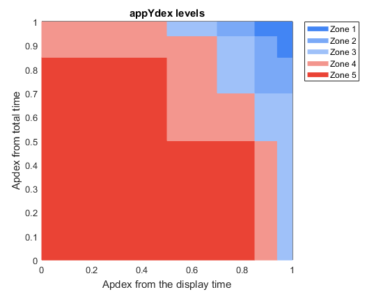
Picture 1 : Satisfaction levels of the appYdex given by the Apdex.
The plan is divided in sub spaces. Every f value can be framed for every given pair x,y. For every zone n (cf table1), minn is its minimum value and maxn its maximum value. Example : For zone 1, min1 = 0,94 et max1 = 1
Let us define En as the group of the x,y belonging to A such as f(x,y) is included in the zone n :
\(E_n=\ \left\{x\ \in A,\ y\in A,\ {min}_n\le f(x,y)\le{max}_n\right\}\\\)
Note : the limits can change zones in the requirement 5. In thiscase, it must be checked that the En constitute a partition of the original space.
\(\bigcup_{n=1}^{5}{En=A^2}\\\)
According to the previously defined limits :
\(E_1=\ \left\{x\ \in A,\ y\in A,\ \ \left(x\geq0,94\ et\ y\geq0,85\right)\ ou\ (x\geq0,85\ et\ y\geq0,94\ )\right\}\)
\(E_2=\ \left\{\ x\geq0,94\ et\ y\in[0,7\ ;0,85[\right\} \cup\ \left\{\ x\in[0,85\ ;0,94[\ et\ y\ \in[0,7\ ;0,94[\right\}\ \cup\ \left\{x\ \in[0,7\ ;0,85[\ et\ y\ \geq0,94\right\}\)
\(E_3=\ \left\{x\geq0,94\ et\ y\ <0,7\ \right\}\cup\left\{x\ \in[0,85;0,94[\ et\ y\ \in[0,5;0,7[\ \right\} \\ \cup\left\{x\ \in[0,7;0,85[\ et\ y\ \in[0,7;0,94[\ \right\}\cup\left\{x\ \in[0,5;0,7[\ et\ y\ \geq0,94\ \right\}\)
\(E_4=\ \left\{x<0,5\ et\ y\geq0,85\ \right\}\cup\left\{x\ \in[0,5;0,7[\ et\ y\ \in[0,5;0,94[\ \right\} \\ \cup\left\{x\ \in[0,7;0,85[\ et\ y\ \in[0,5;0,7[\ \right\}\cup\left\{x\ \in[0,85;0,94[\ et\ y\ <0,5\ \right\}\)
\(E_5=\ \left\{x<0,5\ et\ y<0,85\right\}\cup \left\{x\ \in[0,5;0,85[\ et\ y<0,5\ \right\}\\\)
Throughout the rest of the document, we’ll be talking about plan’s vectors. To simplify it, for a vector v, xv and yv will be its coordinates. The model function is based on the idea that the further a point is the more satisfying it gets. The distance function is defined as followed in the real numbers plans :
\(\forall\ u\in\ R^\mathbb{2}\ ,\forall\ v\in\ R^\mathbb{2}\ ||uv||=\ \sqrt{\left(x_u-x_v\right)^2+\left(y_u-y_v\right)^2}\\\)
This function must now be adapted to respect the previously defined zones. Let O be the origin,
\( x_O=0\ et\ y_O=0\ \ f(O)=0\)
The model function is configured according to the zones (n being the index of the zone in question). For every zone:
- mn the point in En that is the closest to O
- Mn the point in En that is the furthers away from O
Thus :
\(\forall\ p\in\ E_n,\ ||PO||\geq\ ||Pm|| \\ \forall\ p\in\ E_n,\ ||PO||\le||PM|| \\\)
Note : There are potentially several m and/or several M, but it does not make any difference since the distances and not the coordinates of the points that intervene in this calculation. The following function allows to strictly respect the boundaries. :
\(f_n\left(P\right)=f_n\left(m_n\right)+\frac{\ ||OP||-||Om_n||}{\ ||OM_n||-||Om_n||}\left(f_n\left(M_n\right)-f_n\left(m_n\right)\right) \\\)
Which gives :
\(f_n\left(mn\right)=f_n\left(m_n\right)+\frac{\|| Omn|| -|| Om_n|| }{\ || OM_n|| -|| Om_n|| }\left(f_n\left(M_n\right)-f_n\left(m_n\right)\right) \\ f_n\left(mn\right)=f_n\left(m_n\right)\\\)
\(f_n\left(M_n\right)=f_n\left(m_n\right)+\frac{\ ||OMn||-||Om_n||}{\ ||OM_n|| -||Om_n||}\left(f_n\left(M_n\right)-f_n\left(m_n\right)\right)\\ f_n\left(M_n\right)=f_n\left(m_n\right)+\left(f_n\left(M_n\right)-f_n\left(m_n\right)\right) \\ f_n\left(M_n\right)=f_n\left(M_n\right) \\\)
Yet, by definition :
\(\forall\ P\in\ A^2,\ \ ||OMn||\geq\ ||OP||\geq||Om_n|| \\\)
Which leads to :
\(\forall\ P\in\ A^2,\ \ f_n\left(M_n\right)\geq\ f_n\left(P\right)\geq\ f_n\left(m_n\right) \\\)
This expression can be reduced to :
\(f_n\left(P\right)=f_n\left(m_n\right)+\ \frac{\ ||OP||}{\ ||OM_n||-||Om_n||}\left(f_n\left(M_n\right)-f_n\left(m_n\right)\right)-\frac{||Om_n||}{\ ||OM_n|| -||Om_n||}\left(f_n\left(M_n\right)-f_n\left(m_n\right)\right) \)
\(f_n\left(P\right)=||OP||\ \frac{\ \left(f_n\left(M_n\right)-f_n\left(m_n\right)\right)}{\ ||OM_n||-||Om_n||}+\frac{f_n\left(m_n\right)||OM_n||-f_n\left(m_n\right)||Om_n||-||Om_n||f_n\left(M_n\right)+||Om_n||\left(m_n\right)}{\ ||OM_n||-||Om_n||}\)
\(f_n\left(P\right)=||OP||\ \frac{\ \left(f_n\left(M_n\right)-f_n\left(m_n\right)\right)}{\ ||OM_n||-||Om_n||}+\frac{f_n\left(m_n\right) ||OM_n||-||Om_n||f_n\left(M_n\right)}{\ ||OM_n||-||Om_n||}\)
Giving the following result :
\(f_n\left(P\right)=||OP||a_n+b_n \\ avec\ a_n=\ \frac{\ \left(f_n\left(M_n\right)-f_n\left(m_n\right)\right)}{\ ||OM_n||-||Om_n||}\ et\ b_n=\frac{f_n\left(m_n\right) ||OM_n||-||Om_n||f_n\left(M_n\right)}{\ ||OM_n||-||Om_n||}\\\)
The model can be represented in the space (x,y,z) with :
- x, the Apdex score of the beginning of display
- y, the Apdex score of the total loading time
- z, f(x,y)

Picture 2 Spatial representation of the model function
Although it satisfies most of the requirements, this model cannot be used at its current state. Indeed, it shows too important variations in x and in y and around the zone changes. The following step aims to find a polynomial allowing to approximate the most this model while respecting the requirement 6.
4.2 Optimisation of the model
The method of least squares allows to obtain a polynomial² approximating the best the previously seen model. This model showing numerous inflexion points, an acceptable precision is observed from the order 19. The obtained surface can be represented in the space (x,y,z) : 
Picture 3 Spatial representation of the regression result
The results are at first sight relatively close to the model from figure 2 but has notable problems :
- There are irregularities around the zones extremities, especially at x=0 and y=0 and x=1 and y=1.
- There are zones where the z values are clearly decreasing in x and in y.
To resolve these problems, an operation of smoothing is to be done. 
Picture 4 Representation of the final values
Now that the z values are obtained, it is interesting to compare them with those of the model, and particularly the number of point in each of the zones.
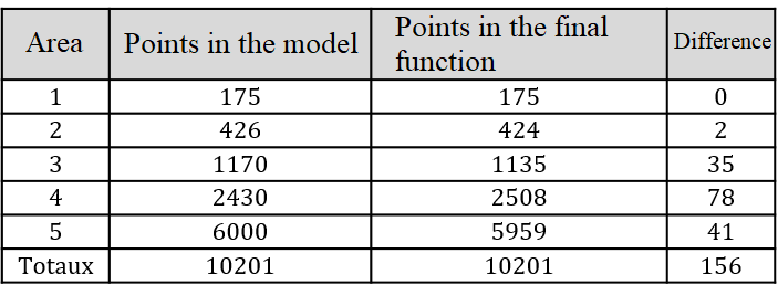 Table 4 : Difference between the model and the final function
Consequently, there are 156 points that are out of their original zone from the model, which represent a bit more than 1% of the total points.
Therefore, this final approximation is close enough to our model to be used as such.